Computer Vision and Human Vision

How does Human Vision work?

Biologically:

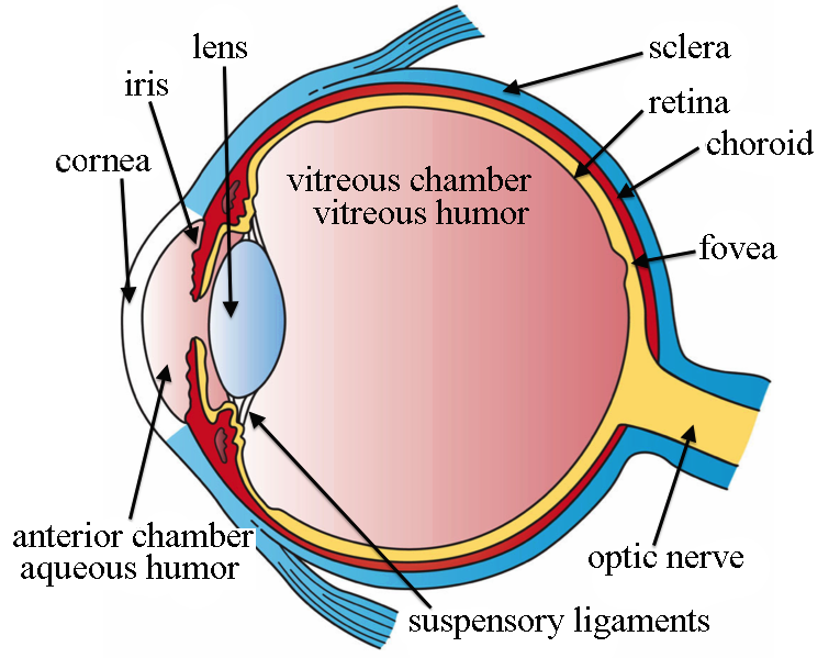
Light initially enters the eye through the cornea (clear front layer of the eye). The cornea is dome shaped and curves the light into a focal point. Some of the light then goes through the pupil and the iris then controls how much light actually passes through into the eye.

Finally, the light passes through the lens, an inner part of the eye, and works with the cornea to focus light into our retina. When light finally hits the retina, photoreceptors(rods and cones) turn the light into electrical signals and transmit them into the brain through the optic nerve. Rods generally pick up a basic light/dark reading while cones require higher brightness levels but pick up red/green/blue. These three colors make up the visible color spectrum.

Our photoreceptors are grouped into clusters and are ‘assigned’ a nerve connecting to our brain. In the brain, our optic center begins to work as we generally receive ~12 discrete images per second. We may only see a blob or splotches of color but our brain helps complete the image with patterns, memories, and context. This may seem slow but our brain is efficient.

Think of your peripheral vision, the resolution is low and generally ‘blob-like’. The images we receive from our peripherals are lower resolution but our brain helps ‘enhance’ our sight. Computers with Convolutional Neural Networks(CNNs) receive images in static grids with constant spatial resolution while the human eye has an eccentricity dependent spatial resolution. Resolution is the highest in the central 5 degrees of visual field but falls off linearly and with increasing eccentricity (our vision gets linearly worse as it gets closer to our peripherals but computers and the images we take with cameras have a consistent resolution).

• Look straight ahead and find the edges of your peripheral vision with your hands and hold up any number of fingers. Your brain will almost convince you that you can see that many fingers being held up since you consciously decide how many fingers to hold up. However, if someone else were to use their hand, it’d we be painfully obvious that we are not actually ‘seeing’ anything recognizable.

How does Computer Vision work?

Pre-processing

• HAAR Cascade Classifier and Haar-like Features

Haar Cascade Classifier is a pretrained model that is a part of OpenCV that provides the detection of faces within images.

Object Detection using Haar feature-based cascade classifiers is an effective and widely used object detection method proposed by Paul Viola and Michael Jones in 2001. It is a machine learning based approach where a cascade function is trained from a large sample of positive and negative images. It is then used to detect objects within other images.

Here we will work with face detection. Initially, the algorithm needs a lot of positive images (images of faces) and negative images (images without faces) to train the classifier. Then we need to extract features from it. Looking into the info within the classifier, we see examples of classifiers and Haar-like features.

<internalNodes>
        0 -1 13569 2.8149113059043884e-003</internalNodes>
      <leafValues>
        9.8837211728096008e-002 -8.5897433757781982e-001</leafValues></_>  

This shows one of the weak classifiers. It’s tree with max depth is equal to 1. 0 and -1 are it’s indexes of left and right child of root node. With indexes less or equal to zero it means that it’s a leaf node. The next number (13569) is the index of feature in the section. And the next number (2.8149113059043884e-003) is the node threshold.

For example, in this weak classifier we need to calculate value of the 13569 feature. Next, compare this value with threshold (2.8149113059043884e-003) and if it’s less than that threshold than we need to add the first leaf value (9.8837211728096008e-002) or add the second leaf value (-8.5897433757781982e-001).

faceCascade = cv2.CascadeClassifier(cv2.data.haarcascades 
                                    +'haarcascade_frontalface_default.xml')

faces = faceCascade.detectMultiScale(gray, 
                                      scaleFactor=1.1,
                                      minNeighbors=6, 
                                      minSize=(60, 60), 
                                      flags=cv2.CASCADE_SCALE_IMAGE)

Here are the standard Haar features. Each feature is a single value obtained by subtracting sum of pixels under the white rectangle from sum of pixels under the black rectangle to quantify an image.

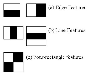
Now, all possible sizes and locations of each kernel (matrix of image) are used to calculate a variety of features (imagine a sliding window moving along the matrix). For each feature calculation, we need to find the sum of the pixels under white and black rectangles. To solve this, they introduced the integral image. However large your image, it reduces the calculations for a given pixel to an operation involving just four pixels.

But with all these features we calculated, they are largely irrelevant. Consider the image below. On the top row, the first feature selected focuses on the property that the eyes are generally darker than the nose and cheeks. The second feature shows that the eyes are darker than the bridge of the nose. However, with thousands of other windows on the cheeks or other places are irrelevant.

To deal with the redundancy, we apply each and every feature on all the training images. For each feature, it finds the best threshold which will classify the faces to positive and negative. Because of errors and miscalculations, we select the features with the smallest error rate (features that most accurately classify the face and non-face images).

The final classifier is a weighted sum of these weak classifiers. The classifiers alone are weak because they can single-handedly classify an image/face, but together the hundreds of weak classifiers forms a strong classifier.

So in application, we take an image, take each 24x24 window, apply our features, and check if we have found a face. This initially seems and is incredibly ineffecient. Thus, optimizations have been added:

In an image, most pixels are part of a non-face region, so it’s a better idea to have a simple method to check if a window is part of a face region. If it isn’t, discard it and don’t process it again. Instead, focus on regions where there can be a face. This way, we spend more time checking possible face regions.

This is where the term Cascade comes in. Instead of applying all 6000 features on a window, the features are grouped into different stages of classifiers and applied one-by-one. Similar to a ‘waterfall’, a cascade of features are applied in stages and are is only continued if the window passes each stage. Typically, the initial stages have less features to further save processing time.

The authors’ of OpenCV’s default detector has 6000+ features with 38 stages with 1, 10, 25, 25 and 50 features in the first five stages. And to demonstrate the times saved, according to the authors, an average of 10 features out of 6000+ are evaluated per sub-window.

Now, as a result, we can quantify the features/faces of images and compare between different images. This data is saved as encodings and used later on to recognize trained faces.

• Gaussian Smoothing/Blur

    image = cv2.imread(image)
    gray = cv2.cvtColor(image, cv2.COLOR_BGR2GRAY)
    smooth = cv2.GaussianBlur(gray, (125,125), 0)

When feeding data into our classifier, a blur is used to reduce ‘noise’ and detail in the image. This is neccesary as extraneous details and background colors/patterns often interfere with both pre-processing and detection.

As seen in the image, the features of the face are largely distinct while the hair, hypothetical background, and unnecesarly sharp edges are faded.

• Grayscaling

Most image processing and CV algorithms use grayscale images for input over RGB images. This is largely because by converting to grayscale, it distincts the luminance and chrominance (Light levels and Color levels). This is helpful because luminance is far more important for distinguishing visual features in an image. Color also doesn’t particularly help identity important features or characteristics of the image (although there are obvious exceptions).

Grayscale images only have one color channel compared to the three in color images (RGB). Thus, the complexity of grayscale images is automatically lower than color images as you can obtain features relating to brightness, contrast, edges, shape, contours, textures, and perspective without color.

Processing in grayscale is generally faster. If we assume that processing a three-channel color image takes three times as long as processing a grayscale image then we can save time by eliminating unneccesary color channels. Essentially, color increases the complexity of the model and in subsequently slows down processing.

Detection

• K-Nearest Neighbors

An introductory explanation of KNN is relatively straightforward. Imagine a neighborhood of two types of families, Blue and Red. We define these two families as classes. When a new house is introduced, we have to define its class and we achieve this by looking at its nearest neighbors.

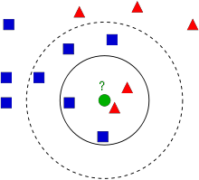
So we see with k=3, we would define the new house as a Red family. With k=4, we could define the new house as a Blue or Red family. This tie demonstrates that there are other factors that should be considered such as distance which leads into the concept of weighted KNN.

Moving onto KNN’s application in OpenCV, the algorithm is able to recognize faces by ‘plotting’ the training faces as our preset ‘houses’ and the face in question as the ‘new house’ waiting to be classified. It’s difficult to visualize this but the algorithm generally bases its detection on the most similar training data and accounts for how similar they are.

• Face Recognition Library

   def compare_faces(known_face_encodings, face_encoding_to_check, tolerance=0.6):
    """
    Compare a list of face encodings against a candidate encoding to see if they match.
    """
    return list(face_distance(known_face_encodings, face_encoding_to_check) <= tolerance)

Compares a list of face encodings against a candidate encoding to see if they match.

Parameters:

• known_face_encodings – A list of known face encodings
• face_encoding_to_check – A single face encoding to compare against the list tolerance – How much distance between faces to consider it a match. Lower is more strict. 0.6 is typical best performance.

Returns:

• A list of True/False values indicating which known_face_encodings match the face encoding to check

At this point, the detection is relatively simple as it compares our trained face data with the detected faces in the test image through ‘encodings’. face_distance returns how similar the trained face encodings are compared to the face_encodings from our input image and the main function then returns true/false depending on the tolerance level.

Adverserial Examples

Based on my research, Adverserial Examples are the next point of interest in Computer Vision as the sheer gap between Human and Computers indicate its importance.

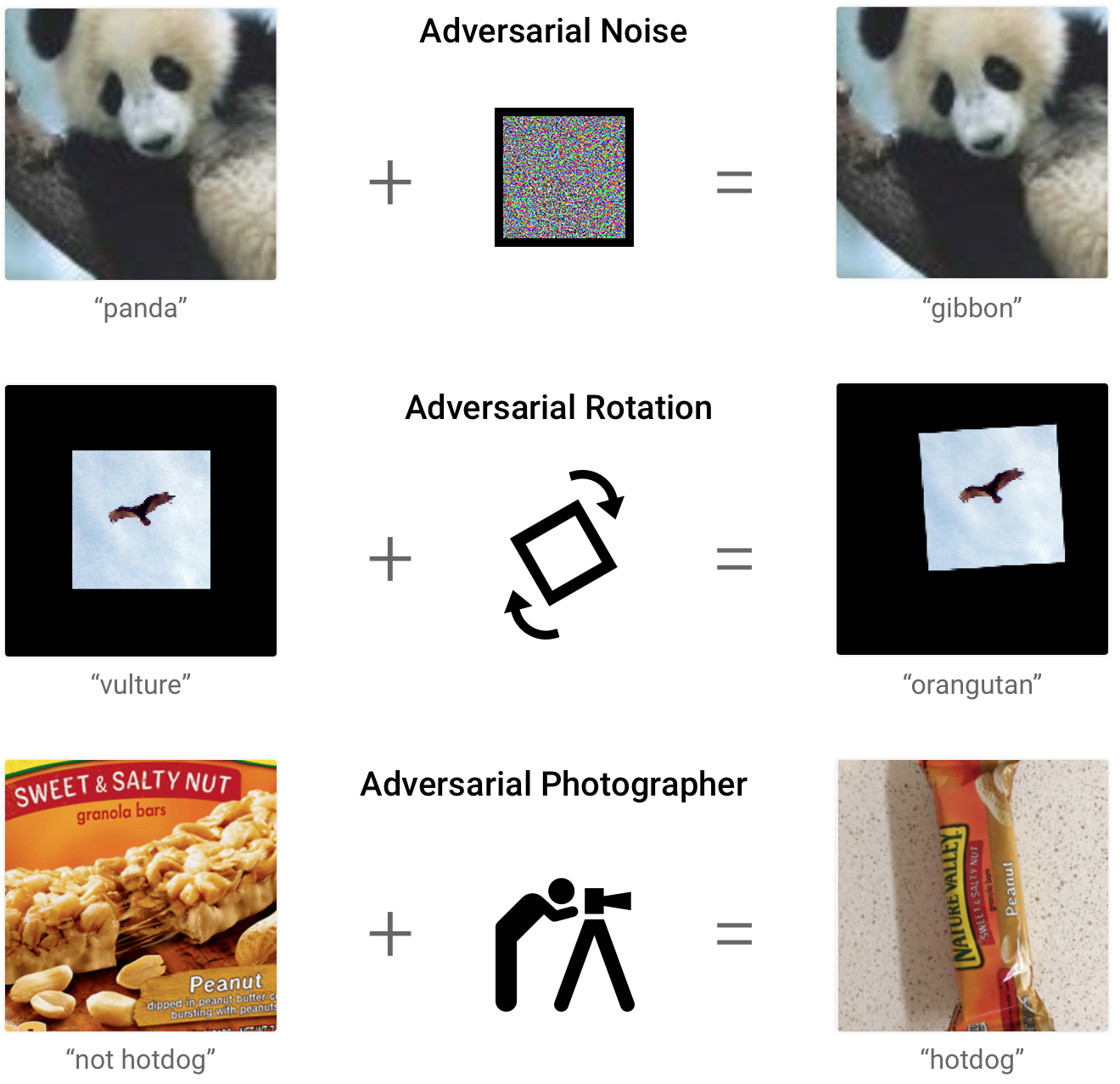
In computer vision, an adversarial example is usually an image formed by making small changes to an example image which result in errors with object recognition. Many algorithms for constructing adversarial examples rely on access to the architecture and parameters of the model to perform gradient-based optimization on the input. In other words, the adverserial examples are finetuned to specifically fool certain recognition algorthims. Therefore, without similar access to the brain, these methods do not seem applicable to constructing adversarial examples for humans. This leads to the question of what “algorithm” does the human brain use? Obviously, this question will remain unanswered for the forseeable future, however, the general methodology of humans can be reasoned.

In this picture, we see minor/imperceptible additions to typical images that subsequently cause misclassifications. The first image is a classic example where adding a small perturbation to an image of a panda causes it to be misnamed as a gibbon.

Note: the ‘static’ added in the panda example is in the final image, it is just imperceptible to humans

Adversial examples highlight the differences between human and computer vision and will be discussed in depth further down. (Biological and Articifial Vision)

Other Methods and/or More Details

• Viola-Jones and Haar - feature based approach

The Viola–Jones algorithm has two stages of training and detection.

In the training stage, the image is turned into grayscale then locates the face within the grayscale image using a sliding box search through the image. Next, it goes to the same location in the colored image. While searching for the face in the grayscale image, Haar-like features. With these features, a value for each feature of the face is calculated, quantifying the face. An integral image is made out of them and compared very quickly in the detection stage.

When detecting, a boosting algorithm named the Adaboost learning algorithm is employed to select a few number of prominent features out of large set to make the detection efficient. Lastly, a cascaded classifier is assigned to reject non-face images where prominent facial features are absent

• Gray Information - feature based approach

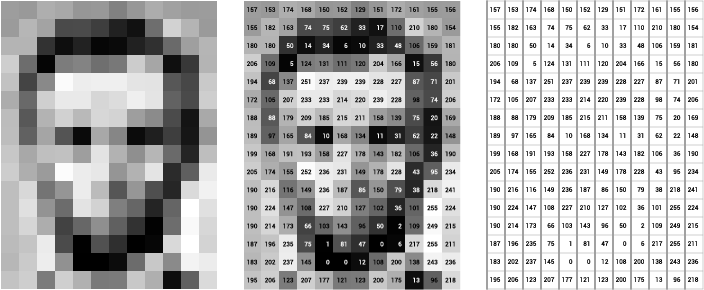
In grayscale images, each pixel in an image represents an amount of light and is quantified into a kernel for analysis. Generally the face shape, edges, and features are darker, compared to surrounding areas. This trend is then used to pinpoint faces from image background or noise and various facial parts from the face.

Analyzing grayscaled images is a two-dimensional process, while RGB is three-dimensional process. Consequently, Grayscaling is computationally less intensive at the cost lowered efficiency as background noise can easily throw off the algorithm. Thus, grayscaling is often used as part of other algorithms as it is a helpful method when paired with other techniques but not as its own face detection algorithm.

• Neural Networks - image based approach

Neural network algorithms are inspired by the human brain’s biological neural network. Neural networks take in data and train themselves to recognize the pattern (for face detection the face pattern). Then, the networks predict the output for a new set of similar faces.

Like the biological human brain, Artificial Neural Networks, ANN, iare based on a collection of connected nodes. The connected nodes are artificial ‘neurons’ and learning patterns in data allows an ANN to have better results with the input of more data.

• Retinal Connected Neural Network (RCNN) - type of ANN

This ANN based on the retinal connection of human eyes was introduced by Rowley, Baluja and Kanade in 1998. The ANN was named the retinal connected neural network (RCNN) as it takes a small-scale frame of the main image to analyze whether the frame contains a face. The algorithm then applies a filter onto the image and is merged with the output into a node. The input is searched, applying a variety of frames to search for a face. The resulting output node eliminates the overlapping features and combines the face features gathered from filtering. Eventually a robust amount of outputs serve as an ANN to recognize faces.

Depending on the constraints or thresholds employed, the process can be sorted out to be more or less reasonable when employing RCNN as an acceptable amount of false positives are reported by the algorithm. However, the process is difficult to apply and can only be used on front facing faces.

Biological and Artificial Vision

• Similarities:

Recent research has found similarities in representation and behavior between deep convolutional neural networks (CNNs) and the human visual system. Activity in deeper CNN layers has been observed to be predictive of activity recorded in the visual pathway of primates. Certain models of object recognition recorded in the human cortex closely resembles many aspects of modern CNNs. Furthermore, researches showed that CNNs are predictive of human gaze fixation. Furthermore, psychophysics experiments have compared the pattern of errors made by humans, to that made by neural network classifiers. While comparably crude, these similarities indicate a start to matching the human’s ocular superiority.

• Differences:

Human advantage does not stem from our vision itself, we actually miss out on a lot of forms of light, however, our processor (brain) is unimaginably advanced. The power of brain is highlighted in several areas.

Differences between machine and human vision occur immediately in the visual system. Images are typically presented to CNNs as a static rectangular pixel grid with constant spatial resolution. The human eye on the other hand has an eccentricity dependent spatial resolution. Resolution is high in the fovea, central 5 degrees of our vision field, but falls off linearly.

Thus, a perturbation in the periphery of an image (this is common in adversial examples) would be undetectable by the eye, and thus would subsequently have no impact on humans. This trend suggests that humans do not fall for adversial examples because our vision itself is trained with adversial examples from birth. Our brain learns to classify ‘perturbed’ versions of objects in our periphery regularly.

Furthermore, there are more major computational differences between CNNs and the human brain. All the CNNs we consider are fully feedforward architectures, while the 3 visual cortex has many times more feedback than feedforward connections. The importance of feedback is discussed by Bruno A Olshausen in great detail. In short, feedback is vital in several fields of engineering and programming and the large usage of feedback loops in our ocular system should be explored.

Thus, due to these differences, humans generally make mistakes that are fundamentally different than those made by deep networks. Also, our brain does not treat a scene as a single static image, but explores it with eye movement and context. Regardless, the general superiority of the human visual system give a path towards higher quality computer vision implementations.

Game Setup

Find all code here -> https://github.com/marvinhcheng/facial_recognition_game

Currently, the dlib library is only usable to me in a Conda environment so the facial recognition program is currently written in a jupyter notebook. Download all attached files and run the facial_rec.ipynb file in a Anaconda Prompt using the following command:

jupyter nbconvert --to notebook --inplace --execute facial_rec.ipynb

This wil create your “face_enc” file which contains the dictionary of names/faces. To add new faces to recognize, input training data into a new folder inside the “faces” folder. Make sure to name the new folder with the name of the new face.

Currently, the game’s images are hand picked with the location of the face hardcoded.

To launch the game use the following command:

jupyter nbconvert --to notebook --inplace --execute game.ipynb

Note: The program can be launched from the notebook itself rather than command line if preferred.

If running into errors, note that the latest version of Conda needs to be installed

conda update -n base -c defaults conda

Sources

Research

https://proceedings.neurips.cc/paper/2018/file/8562ae5e286544710b2e7ebe9858833b-Paper.pdf

https://www.mdpi.com/2079-9292/10/19/2354

http://www.rctn.org/bruno/papers/CNS2010-chapter.pdf

https://directorsblog.nih.gov/2022/04/12/human-brain-compresses-working-memories-into-low-res-summaries/

https://www.mdpi.com/2079-9292/10/19/2354/pdf

https://citeseerx.ist.psu.edu/viewdoc/download?doi=10.1.1.70.2367&rep=rep1&type=pdf

https://www.cv-foundation.org/openaccess/content_cvpr_2013/papers/Dean_Fast_Accurate_Detection_2013_CVPR_paper.pdf

http://www.pyoudeyer.com/

http://people.csail.mit.edu/mrub/vidmag/

https://www.nei.nih.gov/

https://docs.opencv.org/4.x/

Facial Recognition Game

https://www.pygame.org/docs/

https://towardsdatascience.com/building-a-face-recognizer-in-python-7fd6630c6340

https://www.mygreatlearning.com/blog/face-recognition/